Casino Games Online › Card Games › Poker › Poker Variance Explained Using a Simple Example

Variance Explained Using a Simple Example

A simple and illustrative example of variance calculation and its practical meaning and utilization. We will calculate expected profitability (in a way that can be applied to operation of any game or to the game of poker) and variance as possible deviations from the expected profit. After that you will be e.g. able to answer the question "How many hands do I have to play not to lose a dollar with the 99% likelihood?"

What Is Variance

Variance is a statistical measure that shows how the short-term earnings deviate, or may deviate, from the expected long-term average profitability. The more hands are played by a player, the more his profitability (measured e.g. by ROI – Return of Investment) gets crystalized.

Hence the poker player may expect some rate of profitability with some sort of likelihood. There may be a period of bad luck, when his profitability is lower than expected (that is lower than his long-term average). The phenomenon is called the downswing. However he may also be lucky and earn more than the expected average. In this case we talk about the upswing.

The frontiers between which the player's profit moves are called the variance (VAR). The basic information on variance, but also on the way how the good or bad luck may be measured, you can find on the page Variance & Dollar EV Adjusted. This article will show the step-by-step calculation of variance and give you a better understanding of its meaning and use in practice. If this is a new topic to you, then you will be certainly enriched.

The Example or How to Get the Variance Right

Imagine that we took a simple coin and played the following two simple games with it.

Game #1: I will flip the coin. If the "heads" comes out, I will give you $1, and if the "tails" comes out, you will give me $3. At first sight it is obvious that it is a good business for me, but we will get to the point later on.

Game #2: It is coin flipping again, but this time, to make it more interesting, I will have to toss the tails three times in a row. If I manage to do so, you will give me $15, and if I fail, I will give you $1 for each unsuccessful attempt (that is when the heads comes out straight away or after one tails or after two tails in a row).

1. Calculation of Expected Profit or Value (EV)

As for the Game #2 we can see that it is not so easy to determine by eye-balling whether the game is advantageous or not. The decision making, which of the games is better from the long-term prospective, will be aided by the Expected Value (EV), which is a sort of an estimate of a mean profitability of both games (a long-term average). To arrive at the EV we also need to determine the probabilities of winning and losing in both games. The probabilities serve as the weights for possible dollar profits or losses.

Very briefly: the odds of winning and losing in the first game are "Fifty-Fifty", thus the probabilities are equally (1/2) = 0.5. As for the 2nd game, I need to toss the tails 3 times in a row. The probability of managing so is 0.5 × 0.5 × 0.5 = 0.125 (or 12.5%, if you like). The probability of losing is the remainder from one (100%), thus 0.875 (or 87.5%). Now we have everything we need to calculate the expected profit (EV) of both games:

Game #1: EV = 0.5 × $3 + 0.5 × (−$1) = $1.5 − $0.5 = $1.

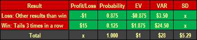
Game #2: EV = 0.125 × $15 + 0.875 × (−$1) = $1.875 − $0.875 = $1.

One more comment on the calculations above: the probability of winning times the profit + the probability of losing times the loss.

Several things arise from the calculations. First, the expected value is positive (+EV), hence both games are advantageous for me (or their operator) in the long run. If I found somebody willing to play them with me, then I would earn in average a dollar out of each toss. (Please note that in terms of the Game #2 we can talk about one attempt or one round that consist in the successful toss of the three tails in a row and in any other failure to do so.)

2. Variance Computation (VAR)

It was the intention of this example that the expected value or profit (EV) of both games was $1. Although we can feel that the Game #1 is somehow more stable and that the deviations in earnings in the Game #2 are more likely. That is what variance (VAR) is all about. It shows the dispersion of the values around the expected value (EV) on both the negative and the positive side. Let us compute the variance. Again, it is not a too big deal, perhaps the explanatory comments below will be helpful.

Game #1: VAR = 0.5 × ($3 − $1)² + 0.5 × (−$1 − $1)² = $4.

Game #2: VAR = 0.125 × ($15 − $1)² + 0.875 × (−$1 − $1)² = $28.

Let us stop at the variance calculations right away. Why they are calculated like that and what do they mean? First we deduct the expected value (EV) from each individual value—that is we deduct the expected profit from all possible profits and/or losses (we have got only one profit and one loss). It shows how much they deviate from the mean value (EV).

As for the Game #1 those are the expressions ($3 − $1) a (−$1 − $1). Then we square the expressions (it will be explained why): ($3 − $1)² a (−$1 − $1)². And finally we multiply the squared expressions by their probabilities (again they serve as weights—in the first game they are equal and thus could be omitted, but in the 2nd game the weights play their part). Now why have we squared them? Simply to prevent the positive and the negative values from eliminating each other. Look what would happen if the differences between the values and the expected value were not squared:
VAR = 0.5 × ($3 − $1) + 0.5 × (−$1 − $1) = 0.5 × $2 + 0.5 × (−$2) = $1 − $1 = $0.
It would suggest that the variance (or the dispersion around the mean) is null, which is not true.

3. Determination of Standard Deviation (SD)

The deviation from the mean value (EV) is determined by the statistical measure known as Standard Deviation (SD). The standard deviation (SD) is nothing else than a square root of the variance (VAR). Can you notice the connection with the previous chapter? First of all, all differences from EV were squared, hence the negative values turned into the positive values. Now we take the square root of the sum of all these (positive) values. By that we arrive at the standard deviation around the EV on both sides (+/−).

Game #1: SD = square root of 4$ = $2.

Game #2: SD = square root of 28$ = $5.29.

Practical Use of Variance

How can we utilize the general knowledge and specific calculations of the expected profit (EV), variance (VAR) and standard deviation (SD) from the mean value? First let us have a small recap so that we can come back to it if needed.

Table 1: Summary of the Game #1

Coin flipping Game #1 - EV, VAR, SD

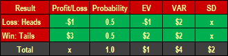
Table 2: Summary of the Game #2

Coin flipping Game #1 - EV, VAR, SD

Let Us Play 100 Rounds and See What Happens

Imagine that we want to play 100 tosses (rounds or attempts). If we expect to earn a dollar in average on each round of the game, then after 100 rounds we are supposed to earn 100 dollars in average. "We are supposed" does not mean that we will earn $100. We can earn more or less and as we will see 100 rounds is not large enough number for our expected earnings to take full effect.

Game #1:

EV = 1$ × 100 rounds = $100 VAR = $4 × 100 rounds = $400 SD = square root of $400 = $20

Note: SD can also be calculated as the square root of ($4 × 100), that is square root of $4 times the square root of 100 rounds = 2 × 10 = $20.

Game #2:

EV = 1$ × 100 rounds = $100 VAR = $28 × 100 rounds = $2800 SD = square root of $2800 = $53

How to Utilize the Standard Deviation

Now the three-sigma rule comes into existence. No need to panic about statistics, the examples below will manifest themselves and you will get the understanding of how to use the SD. In statistics sigma (σ) is a Greek letter used for the standard deviation (SD) and sigma square (σ²) is used for the variance (VAR). Let us keep it simple and stick to our abbreviations SD and VAR as they are virtually the same. However this is what the three-sigma rule tells us:

Almost 70% of values (precisely 68.27%) are found in the distance lower than one SD from the mean expected value (EV), that is almost 70% of values lie in the interval (EV − SD; EV + SD),
About 95% of values (precisely 95.45%) lie in the interval (EV − 2 × SD; EV + 2 × SD), and
About 99% of values (precisely 99.73%) lie in the interval (EV − 3 × SD; EV + 3 × SD).

We will be interested mainly in the last two intervals, that is 95% and 99%. What are they good for? It will be clear by the following calculations and comments.

Game #1:

EV = 1$ x 100 rounds = $100 VAR = $4 × 100 rounds = $400 SD = square root of $400 = $20

95%
min = EV − 2 × SD = $100 − 2 × $20 = $60 max = EV + 2 × SD = $100 + 2 × $20 = $140

What does this say? I expect an average profit of $100 (EV), that is still the same, but the real profit may–with 95% likelihood—move between the minimum (min) and the maximum (max). Hence with the 95% likelihood my worst result will be +$60 (downswing), but if I was lucky (upswing) I could earn up to +$140 (in both cases in comparison to the expected profit $100).

If I want to raise the rate of likelihood to 99% (that is almost certainty = 100%), I have to count on the fact that the interval will be larger as well (as I add or deduct the triple of the SD compared to the double of the SD in terms of 95% interval).

99%
min = EV − 3 × SD = $100 − 3 × $20 = $40 max = EV + 3 × SD = $100 + 3 × $20 = $160

Now the conclusion is the following. Again, I am about to earn $100 dollars in average in 100 rounds (EV). With the 99% likelihood my real earnings will be found in the range of +$40 (the worst case scenario, the worst downswing) to $160 (the best scenario) as compared to the expected earning of $100.

That is the variance and it is essential to realize that variance's effect can go both directions (both plus and minus or both lower and higher than expected average). This first game of coin flipping, when I receive $3 and pay $1 with the same odds of winning and losing, is so advantageous that 100 rounds is enough for me to be in the plus with the 99% likelihood. Let us have a look at the second game, where the variance is much bigger.

Game #2:

EV = 1$ × 100 rounds = $100 VAR = $28 × 100 rounds = $2800 SD = square root of $2800 = $53

95%
min = EV − 2 × SD = $100 − 2 × $53 = −$6 max = EV + 2 × SD = $100 + 2 × $53 = $206

The expected profit (EV) is the same $100, but due to the bigger variance my real earnings with 95% likelihood will lie in the interval −$6 to +$206. It means that in worst case scenario (i.e. if I caught a terrible downswing) I could even lose, even though I was supposed to win $100 in the long-term average! On the side, the upswing could earn as much as $206 (again as compared to the expected $100).

99%
min = EV − 3 × SD = $100 − 3 × $53 = −$59 max = EV + 3 × SD = $100 + 3 × $53 = $259

What is the conclusion for the interval covering 99% of the values? After 100 rounds my earnings with the 99% likelihood will range from minus $59 to plus $259. It means that if I was unlucky (downswing), I could lose up to $59. On the other side if I had extraordinary luck (upswing), I could win up to $259. Both the min and the max values are to be compared to the expected average profit of $100 out of 100 rounds played.

What can I do in order not to lose a single dollar with the 99% likelihood?

My strategy, or in this case the operation of the coin flipping game is advantageous as the numbers favor me and according to the assumption I should earn 1 dollar in average out of each round played. A hundred of rounds, however, proved to be insufficient for the advantage to strike in full and I can even end up in the red. The solution is to raise the number of rounds played! The more round, the better as the earning will convert to the expected value. There is a break point after which I cannot lose (with the 99% likelihood) and I am about to win $1 in average out of each round played. The possible negative impact of the variance will be suppressed by the greater number of rounds.

How many rounds do I need not to lose a dollar with the 99% likelihood?
The break point number of rounds (n)is when the minimum profit is zero (min = 0). The condition is the following:

n × EV − 3 × square root of (n × VAR) = 0. EV and VAR in this formula apply to one round only and they are multiplied by the number of rounds n. After the adjustment we arrive at the minimum number of games n that need to be played:

n = 9 × VAR ÷ EV² and after inputting the concrete values

n = 9 × $28 ÷ $1² = 252 rounds.

It is needed to play at least 252 rounds so that the profit of the 2nd coin flipping game is null at worst. Let us verify it:

Game #2, 252 rounds

EV = 1$ × 252 rounds = $252 VAR = $28 × 252 rounds = $7056 SD = square root of $7056 = $84

99%
min = EV − 3 × SD = $252 − 3 × $84 = $0 max = EV + 3 × SD = $252 + 3 × $84 = $504

→ How to calculate poker variance for 9 player Sit and Go.

Findings

The two simple coin flipping games demonstrate the meaning of variance not only in poker. Both games are favorable for their operator as they would bring the same expected long-term average profit $1 out of each round played. Of course it does not mean that each individual round (or toss of the coin) would end up with this result, but in the long run, that is after a big enough number of rounds played, the profitability of the games operator would head towards these expected result.

A player's results (or earnings) in the long run tend to oscillate closely around the mean value (or average). However in the short run the deviations occur. The variance shows how big they can be. The bigger the variance (deviation), the greater is the risk that a poker player may end up with losses. However the variance takes effect in both directions and you can earn more than average in the short run.

An operator of any game with the positive expected value (+EV), or a poker player, who has a good strategy, that is he plays good poker (maximizes EV) and maintains a long-term profitability (+ROI), must ultimately be profiting in the long-term period. The second coin flipping game showed that the bigger is the variance, the more rounds it is need to play for the strategy, or the advantage, to prevail with the high rate of likelihood (95% or 99%). It is desirable to strive for the maximum EV and as low as possible VAR.

If you are an entrepreneur running your own business or come in touch with sales management or you buy stocks, you can find under these links how the expected value and the variance (VAR = risk) can be utilized in these areas. The principle is the same as described on this page.